
Rigorously hedging against tail latency
2026-08-31
I saw a talk at CppCon 2024 delivered by a friend of mine on request latency outliers, find it on YouTube here.
The talk proceeds roughly as follows:
- A very small number of requests to a service are very slow
- We find out what's going on with those requests and fix it
- Everyone is happy, we experience some fun C++ map implementation comedy and go home satisfied.
But let's suppose we're in a worse situation, where:
- A very small number of requests are very slow
- We've investigated and cannot reliably reproduce anything
- We want to fix the tail latency anyway!
An out of the box solution in gRPC is request hedging. The configuration we'll explore is where your client sends $n$ requests, waits for the first response, then cancels the rest.
Observe that latency must be positive, so a natural idea for a latency distribution is a log normal distribution. That is, we'll say that if latency is $T$, then $\log(T) \sim \mathcal{N}(0,1)$. Some questions:
What's the distribution of latencies of the hedged request?
Does this change if the latency has a different distribution? Does lognormal even make sense?
What do the limits as $n$ goes to infinity look like? What distribution does infinitely hedged request latency have under these assumptions? And what about in the real world?
I haven't been able to find rigorous statistical descriptions of these hedging strategies online. I discuss queueing theory a bit below, which is unsatisfying, but maybe I haven't dug deep enough yet.
Computing the hedged distribution
As usual, these blog posts aren't tutorials. Read the guide if you want some insight into gRPC's request hedging. It supports more than the configuration I'll describe here.
I also assume knowledge of statistics. For a course in statistics, please enroll at your nearest university.
Suppose a request's latency $T$ is log-normally distributed, with $\log(T) \sim \mathcal{N}(0,1)$. We send $n$ requests and call the latency for the $i$th request $T_i$, with $\log(T_i) \sim \mathcal{N}(0,1)$, where the $T_i$ are independent.
It's a general result that for $X_i$ independent and identically distributed, with CDF $F$, then the CDF $F_n$ of $\min_i(X_i)$ is $1-(1-F(x))^n$. Proving this is an exercise for the reader (saying this is totally rigorous, do not send me complaints). Similarly, the max would be $F(x)^n$.
The hedged latency distribution $H_n$ is $\min(T_1, \dots, T_n)$.
$$\log(H\_n) = \log(\min(T\_1, \dots, T\_n))$$
$\log$ is increasing, so this is $\min(\log(T_1), \dots, \log(T_n))$.
Writing $\Phi$ and $\phi$ for the standard normal CDF and PDF, we have
$$P(\log H\_n \le y) = 1-(1-\Phi(y))\^n$$
where the intuition is that for $\log H_n$ to be less than $y$, this happens if and only if at least one of $\log T_i$ is less than $y$, i.e. not all of them are more than $y$, and those are all allegedly normal.
The PDF is then (by differentiating):
$$f\_{\log H\_n}(y) = n(1-\Phi(y))\^{n-1}\phi(y).$$
We can plot it for various values of $n$ to build some intuition before we prove some facts.
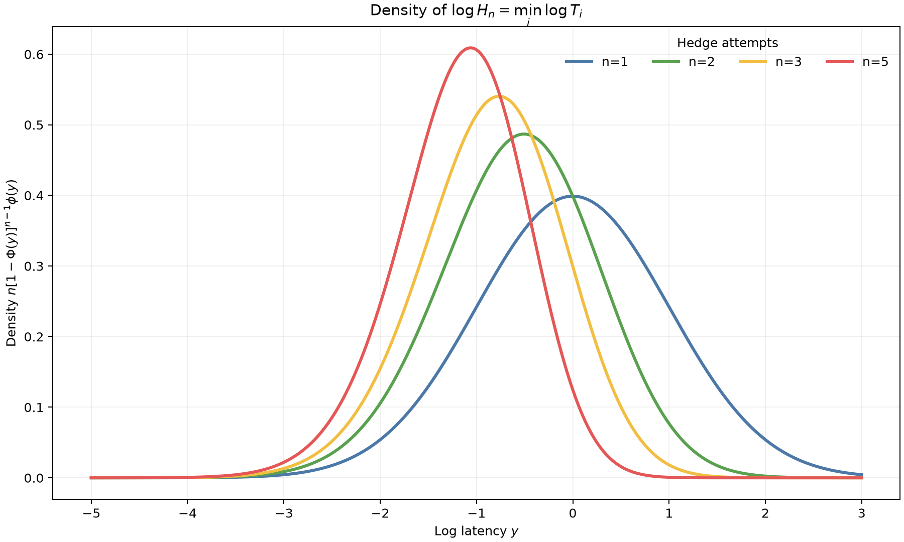
It's clear from looking at this that the hedged distribution isn't lognormal. It isn't just moving to the left, it's now asymmetric, the tail on the left is flatter and the distribution is narrower.
For any fixed $x>0$, $F(x)>0$, so
$$\lim\_{n \to \infty} 1-(1-F(x))\^n = 1.$$
For $x \le 0$, every $F_n(x)$ is zero, so $H_n$ converges in distribution to zero. This cannot be uniform: at $x=0$ every $F_n$ is zero but the CDF of the constant zero random variable is one.
This makes sense - requests may have latency arbitrarily close to zero. So with more hedging, the hedged latency distribution gets more and more squeezed towards zero (or the log shifts towards larger negative values). This is the intuitive answer I was referring to at the start.
But hang on a moment - if you sent an infinite number of requests to an actual server, all at the same time, that would probably cause a lot of queueing (infinity is a big number), or cause some kind of global system slowdown. Infinite hedging should not cause the service time to go to zero - our modelling is too simple.
Let's ask and answer an easier question first: why does the variance decrease? i.e. why is the distribution getting narrower? This is a key property of hedging, it allows you to reduce variance.
Why does variance decrease?
I'm not aware of a closed form for the variance of $N = \min_i N_i$ for $N_i$ independent, normal, identically distributed.
It is relatively easy to prove that the variance of the min of i.i.d. lognormal random variables tends to zero the more you add. I won't pretend I didn't just look it up on Math StackExchange.
This works because lognormal variables have support $(0,\infty)$ and finite second moments. $H_n$ tends to zero and $0 \le H_n \le T_1$, so dominated convergence gives $E[H_n] \to 0$ and $E[H_n^2] \to 0$.
The variance converges to zero as $n \to \infty$. This doesn't by itself prove that it decreases at every single step.
The intuition for this is clear, going from $F(x)$ to $1-(1-F(x))^n$ squashes the right part of the CDF towards 1 faster than the left. This looks more and more like a step function as you increase $n$.
Why not lognormal?
Why model request times lognormally? One answer is that experimentally, things seem to fit that distribution. This explanation is intellectually barren and lazy. Another argument is that delays are the product of many smaller delays.
The argument goes like this:
Delays multiply. Suppose we have delays $d_i$, of some distribution we don't care about, where the $d_i$ are independent random variables.
Then log of the total delay $\log \prod_i d_i = \sum_i \log d_i$ is the sum of a lot of independent variables, central limit theorem, it's normal.
The problem with this is that it's nonsense. Delays don't multiply, they add up!
The log of the total delay isn't $\log \prod_i d_i$, it's $\log \sum_i d_i$. But why even take the log, the total delay is just $\sum_i d_i$, so the total delay is normally distributed - but this is obvious nonsense since it has nonzero density on the whole real line, allowing negative service times.
We must assume more about the $d_i$ to make sense of this.
Wow, it turns out everything we just did was pointless! Fear not, we can think of a better distribution to use, right?
Which distribution should we use?
Is latency different if there are 1 billion qps or 1 qps? Of course it is. To model the effects of load, our model must model the distribution of request arrivals.
A clear contender for modelling time between arrivals is the exponential distribution - it models the time between independent events where the average arrival rate is constant, i.e. the number of arrivals has a Poisson distribution.
We also have to pick a model for service times. You could pick any distribution. Here's an argument for using the exponential distribution:
- It gives lots of nice results
- REALLY nice results!
Really! There are lots of very nice closed form results for this case (exponential arrival and service times, and 1 server), see https://en.wikipedia.org/wiki/M/M/1_queue and other articles on queueing theory.
There's no general answer for this that doesn't make service time assumptions.
Note also that this queueing model is in general useless because service times aren't independent!
And there's another problem, request arrivals are usually not independent, traffic to any real system is usually spiky and correlated with e.g. sports events, news, market events. This means the "constant average arrival rate" assumption behind using the exponential distribution is wrong.
Once you lose independence and don't know the distributions of anything, you can no longer use the nice closed form results and have to measure experimentally.
So let's do an experiment!
Measuring gRPC response times with hedging
I set up a Java gRPC service which does nothing but wait for a random time drawn from various distributions. We'll benchmark it and measure times taken with request hedging for various distributions. The code is here.
This is overkill - I could've simply written a model in a Jupyter Notebook and come up with these same numbers. It's a more satisfying conclusion for me though, after being unable to prove anything.
The benchmark uses a fixed 32 concurrent client requests since we just want to think about service times. The server samples a new independent delay for every attempt and schedules the response without blocking a thread. I used these two distributions:
- $5\text{ms} + \operatorname{Exponential}(20\text{ms})$
- $5\text{ms} + \operatorname{Lognormal}(\log(10\text{ms}), 1)$
The extra 5ms gives gRPC enough time to start every zero-delay hedge before one of them finishes.
The proto file looks like this:
service BenchmarkService {
  rpc Process (BenchmarkRequest) returns (BenchmarkResponse) {}
}
The hedging config looks like this for $n=3$:
{
  "methodConfig": [{
    "name": [{"service": "benchmark.BenchmarkService"}],
    "hedgingPolicy": {
      "maxAttempts": 3,
      "hedgingDelay": "0s"
    }
  }]
}
The first version of the benchmark used JMH iteration averages as though they were individual request times. That was wrong, we need all the individual times if we want to look at a distribution. The fixed benchmark records 5,000 individual calls for each distribution and each value of $n$.
I also added counters to the server for attempts, completed attempts and cancelled attempts. This verifies that gRPC is actually hedging instead of just measuring an unhedged request and producing a very boring result.
Does the experiment match theory?
The solid lines below are measured gRPC latencies and the dashed lines are the theoretical CDFs $1-(1-F(x))^n$.
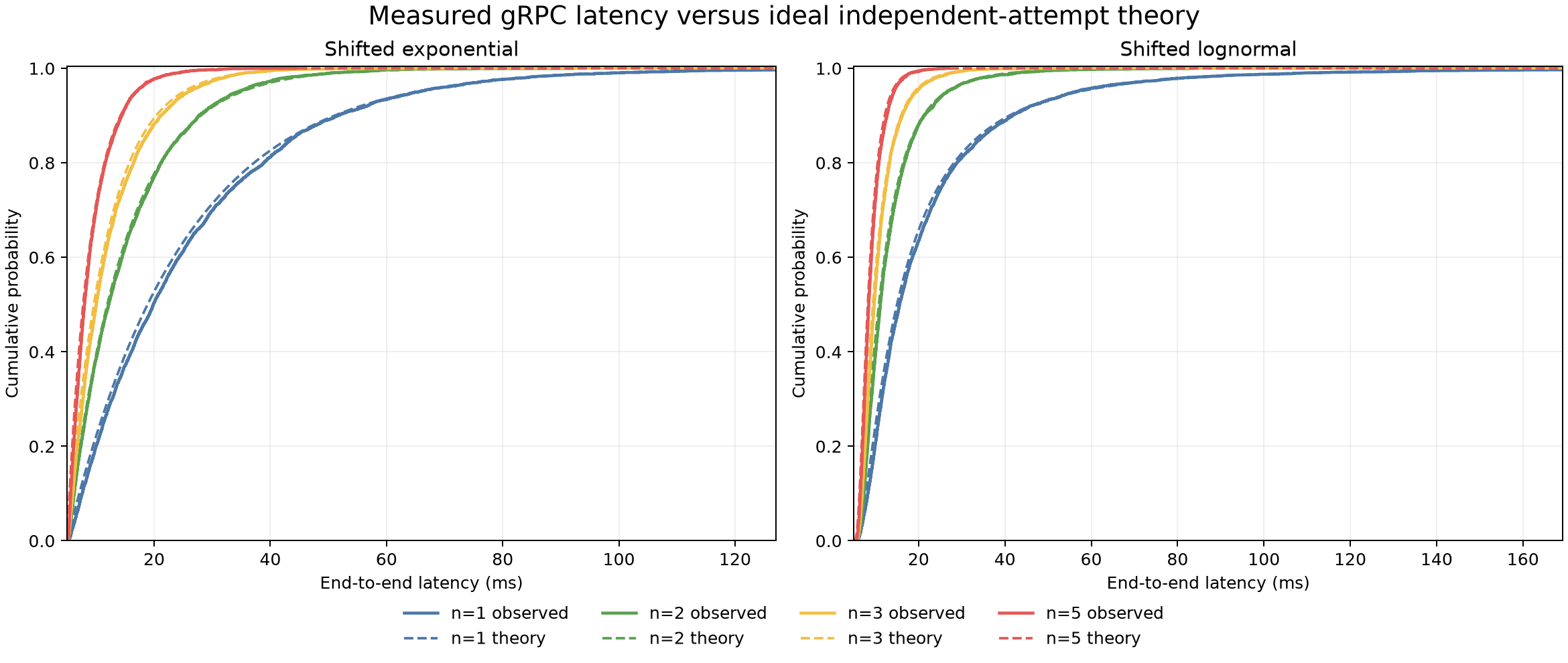
Every measured p50, p95 and p99 is within 1.6ms of the theoretical value. The measured values include gRPC, HTTP/2 and scheduling overhead while the theory only includes the delay sampled by the server, so they shouldn't be exactly equal.
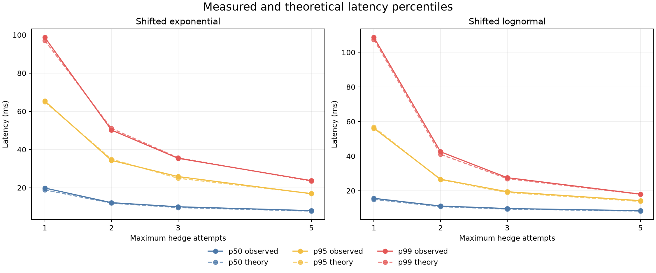
Here are the tail results. "Theory" is the exact p99 of the minimum of $n$ independent service times.
| Distribution | $n$ | Observed p99 | Theory p99 | Attempts/call |
|---|---|---|---|---|
| Exponential | 1 | 98.69ms | 97.10ms | 1.00 |
| Exponential | 2 | 50.19ms | 51.05ms | 2.00 |
| Exponential | 3 | 35.42ms | 35.70ms | 3.00 |
| Exponential | 5 | 23.70ms | 23.42ms | 5.00 |
| Lognormal | 1 | 108.63ms | 107.40ms | 1.00 |
| Lognormal | 2 | 42.50ms | 41.02ms | 2.00 |
| Lognormal | 3 | 27.56ms | 26.98ms | 3.00 |
| Lognormal | 5 | 18.03ms | 17.95ms | 5.00 |
There's a cost, obviously. Zero-delay hedging started exactly $n$ server attempts for every request. At $n=5$, the exponential run cancelled 19,901 of 25,000 attempts and the lognormal run cancelled 19,819. A small number of the losing attempts completed before cancellation reached the server.
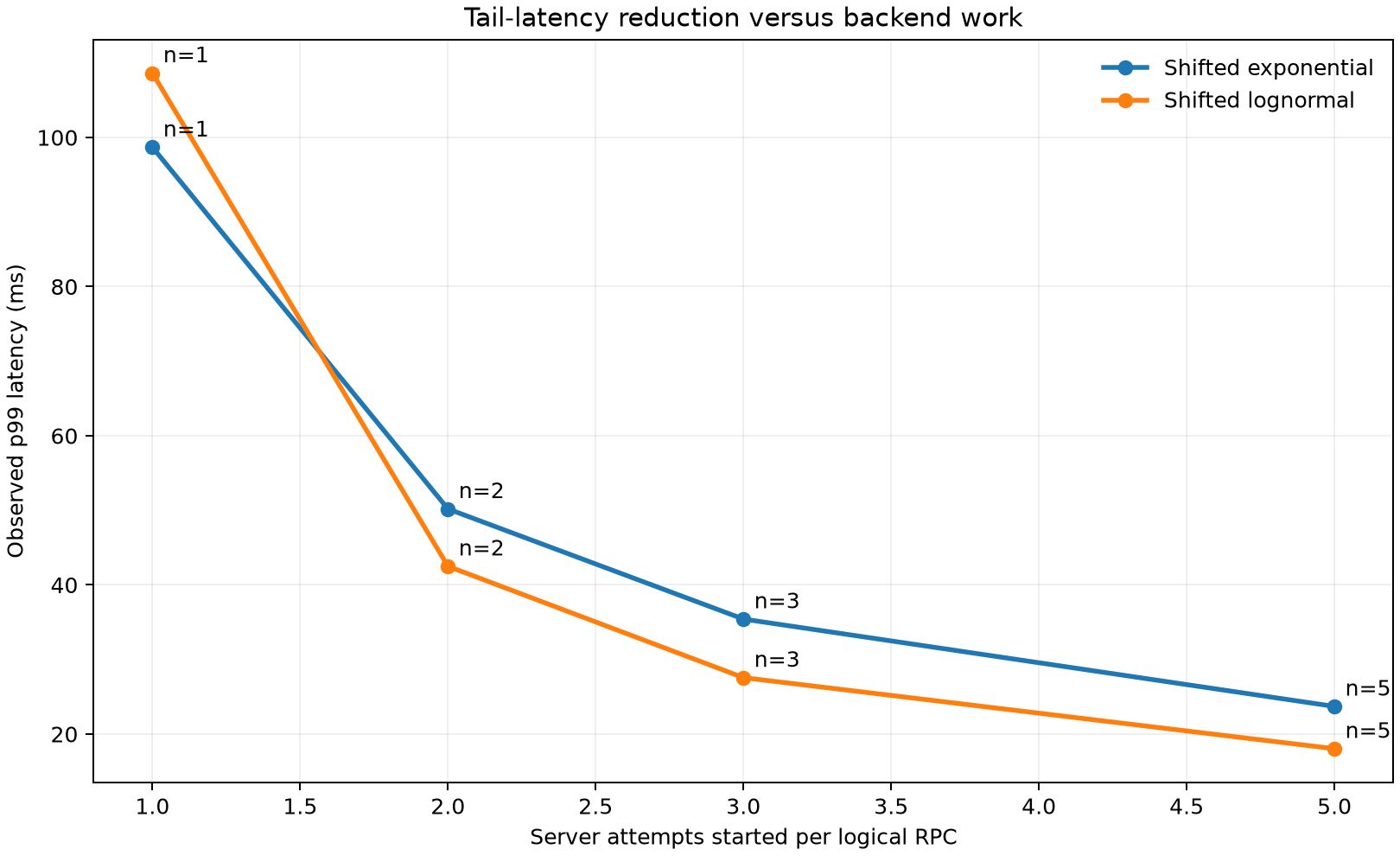
So the simple model was not pointless after all. It predicts the result very well when we deliberately make the assumptions true.
This doesn't mean you should send five copies of every request. Real attempts may be correlated because they share a database or overloaded backend. The extra attempts also consume real resources, cancellation can arrive too late, and the operation must be safe to run more than once.
A delayed second request is less silly than sending five immediately. For example, you could send it around the ordinary p95 latency, targeting the tail without doubling the load for every request. gRPC has throttling and server pushback for similar reasons.
Conclusion
My conclusion here is that it's really tough to model real world phenomena when events are correlated. Theorems that I used to use every day like the trusty old central limit theorem are totally useless.
This actually has real world implications - I build distributed systems subject to spiky load. Far spikier than normal distributions would suggest because sometimes things happen. That means theoretical results are largely useless.
The lesson being that a toy example proves some stuff about exponential distributions working well as a toy model but it doesn't really work that well if you have to actually handle huge, sudden queues. Queueing theory doesn't tell you a closed form for what happens if you try to hedge a request by sending 1 billion requests and taking the first one to return, but I've got a queue for you if you try that - the unemployment queue! Apologies if you didn't get that joke, I'll work on my queue joke timing and delivery.
Let me know if you do discover any closed forms for any of the above!